Mercury’s extreme day-night temperature swings mapped worldwide ahead of BepiColombo

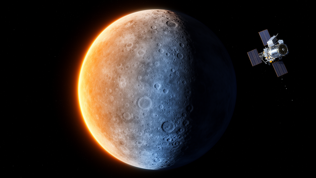
Mercury endures the most brutal daily temperature swing in the Solar System, and a new global modeling study has now charted that thermal rollercoaster across the entire planet in preparation for the European-Japanese BepiColombo mission. Surface temperatures on the innermost planet plunge below 100 K during the long Mercurian night and climb above 700 K at local noon, a cycle driven by the planet’s peculiar 3:2 spin-orbit resonance and its intense solar irradiance. The new work, published in Earth, Planets and Space, delivers planet-wide maps of maximum surface temperature, diurnal temperature amplitude, longitudinal thermal gradients and a thermal stress index designed to help scientists plan and interpret observations from the SIMBIO-SYS instrument suite aboard the BepiColombo orbiter.

Each surface pixel is treated as an independent vertical column of soil, an approximation the authors note is valid at the resolution of their global grid. The model couples this conduction scheme with real topography drawn from the MESSENGER Digital Terrain Model, a global elevation dataset with a spatial sampling of roughly 665 meters per pixel at the equator, so that local slopes and orientations explicitly shape how much sunlight each location receives.

The physics behind the simulation is detailed but grounded in well-established formulations. At the surface, a radiative energy balance determines the temperature: absorbed sunlight, scaled by a bolometric Bond albedo of 0.10 and modulated by the cosine of the solar incidence angle, is offset by thermal emission governed by an emissivity of 0.95 and by heat conducted downward into the ground. The solar flux itself varies along Mercury’s eccentric orbit, computed from JPL ephemeris data with a solar constant of 1361 watts per square meter scaled by the inverse square of the Sun-Mercury distance. Below the surface, the model solves the one-dimensional heat diffusion equation using depth- and temperature-dependent regolith properties: density rises exponentially from 1300 to 1800 kilograms per cubic meter over a characteristic scale height of 0.06 meters, specific heat varies with temperature, and thermal conductivity increases with depth from about 9.22 by 10 to the minus fourth to 9.3 by 10 to the minus third watts per meter-kelvin, reflecting the transition from the insulating, porous uppermost regolith to more compacted material below.

The computational domain extends four meters deep, discretized into 41 layers of roughly 0.1 meters each, with a zero-heat-flux condition at the bottom boundary. Simulations started from a uniform 200 K and were stepped forward in three-hour increments over successive Mercury years until the temperature field settled into a periodically repeating solution.

The resulting maps confirm the striking two-lobed thermal architecture long predicted for Mercury. Two vast equatorial hot regions centered near 0 and 180 degrees longitude reach peak maximum temperatures of about 720 to 730 K. These are the famous hot poles, longitudes that happen to face the Sun directly during perihelion passages, when the planet sweeps closest to the Sun and solar heating peaks, a consequence of the 3:2 spin-orbit resonance that locks specific surface regions into repeated cycles of extreme heating. In between, the so-called cold longitudes near plus and minus 90 degrees see maximum temperatures of only about 500 to 550 K, because the Sun lingers at low elevation angles through most of the solar day there, limiting the absorbed energy.

Latitude imposes an equally strong imprint. Maximum temperatures stay above 600 K across equatorial and mid-latitude zones but fall below 300 K beyond about 70 degrees latitude, dropping to roughly 200 K near the poles. The authors caution, however, that the polar values are the least trustworthy: limited illumination geometry and reduced data accuracy in MESSENGER’s global terrain models at high latitudes mean these zones may suffer from projection artifacts and insufficient photometric correction, so they were excluded from quantitative interpretation. Small departures from perfect longitudinal symmetry in the maps arise purely from topographic modulation of the local solar incidence angle, since the model assumes a uniform albedo and emissivity everywhere.

The diurnal temperature amplitude, defined as the difference between daily maximum and minimum temperature, follows the same double-peaked pattern. Broad maxima of 520 to 550 K occur near the hot-pole longitudes, where perihelion heating produces the largest day-night oscillations, while amplitudes decline smoothly and nearly symmetrically from about 520 K at the equator to below 200 K at the poles. Between 0 and plus or minus 60 degrees latitude, that decline follows an approximately linear gradient of about minus 3 K per degree, a quantitative measure of how solar forcing weakens toward higher latitudes. Regions with amplitudes exceeding 500 K, mainly the equatorial belt around the hot poles, are expected to experience the most intense thermoelastic stress cycling, favoring thermal fatigue, microfracturing and the progressive grinding down of regolith.

To pinpoint where the thermal environment changes most abruptly, the team computed the longitudinal gradient of the diurnal amplitude. Two extended belts of elevated gradients emerge between roughly minus 60 and minus 90 degrees longitude, at the transitions between hot and cold longitudes, where the gradient reaches local maxima of about 100 to 150 K per degree. These belts mark the edges of the hot poles, where the day-night temperature swing changes most sharply because of the alternating pattern of prolonged illumination and darkness imposed by the spin-orbit resonance. By contrast, the 0-degree and plus-or-minus-180-degree longitudes show low gradients, consistent with spatially uniform thermal conditions in areas that remain steadily illuminated or dark for extended periods. From these fields the authors derived a thermal stress index, defined as the diurnal amplitude divided by the length of the Hermean solar day, which quantifies the mean rate of temperature cycling and serves as a first-order proxy for thermally induced mechanical stress. Its global distribution highlights belts of enhanced thermoelastic cycling along the equator and around the hot poles, where rock breakdown and regolith production by thermal fatigue are expected to be most efficient, while high latitudes and dawn-dusk sectors emerge as thermally more stable environments potentially favorable for volatile preservation.

One of the study’s most instructive results is a negative one: local terrain shape barely matters at the planetary scale. Correlating maximum temperature pixel by pixel with slope, roughness, hillshade and aspect derived from the global Mercury elevation model yields uniformly small Pearson coefficients, all below about 0.12 in absolute value, meaning each parameter alone explains well under a few percent of the temperature variance. A multiple linear regression combining all four variables yields a coefficient of determination of only about 0.04, so morphology as a whole accounts for roughly 4 percent of the spatial variability in modeled temperature maxima, even though the enormous pixel count makes the fitted coefficients formally statistically significant. The authors stress that this result reflects their one-dimensional framework, which does not explicitly simulate three-dimensional radiative effects such as mutual shadowing and self-heating, the very mechanisms through which roughness influences local temperatures; the correlations should therefore be read as statistical relationships between the modeled temperature field and terrain descriptors rather than a direct measure of roughness effects. Binned scatter plots reinforce the picture: mean temperature trends vary only gradually with slope and roughness and stay nearly flat against hillshade and aspect, while the vertical scatter at any fixed morphology spans several hundred kelvin. Steeper terrains show slightly different maximum temperatures and rougher surfaces modestly higher ones, but these are second-order adjustments on a thermal regime overwhelmingly governed by latitude and spin-orbit-driven insolation.

For BepiColombo, which launched in October 2018 and is expected to enter orbit around Mercury in late 2026, these products arrive at an opportune moment. SIMBIO-SYS combines a stereo camera, a high-resolution imaging channel and a visible-infrared hyperspectral imager to observe Mercury’s morphology, mineralogy and surface properties, and interpreting those data requires a physically consistent description of the thermal environment. The team positions the global model as a first-order tool for identifying Regions of Interest and prioritizing targets, not for detailed local analysis; once promising areas are selected, dedicated three-dimensional thermophysical simulations, such as the model the group previously applied to Mercury’s polar craters, can capture self-shadowing, mutual radiative heating and other local effects. The modeling tool will be made available to the SIMBIO-SYS community, allowing users to generate customized temperature, amplitude and thermal-stress products for specific regions or observation scenarios as the mission begins its orbital phase.

Subject of Research: Global thermophysical modeling of Mercury's diurnal surface temperature cycle in support of the BepiColombo SIMBIO-SYS mission

Article Title: Global thermophysical characterization of Mercury’s diurnal temperature cycle in support of BepiColombo SIMBIO-SYS

Article References: Cambianica, P., Cremonese, G., Simioni, E., Tullo, A., Bertoli, S., Re, C., Massironi, M., & Martellato, E. (2026). Global thermophysical characterization of Mercury’s diurnal temperature cycle in support of BepiColombo SIMBIO-SYS. Earth, Planets and Space, 78(1), Article 233. https://doi.org/10.1186/s40623-026-02564-y

Image Credits: AI Generated

DOI: 10.1186/s40623-026-02564-y

Keywords: Mercury, BepiColombo, SIMBIO-SYS, thermophysical modeling, diurnal temperature cycle, 3:2 spin-orbit resonance, MESSENGER Digital Terrain Model, thermal stress index, regolith, hot poles, heat conduction, surface temperature maps