WaveLab Studio: Lightweight software for interactive 2D wave propagation experiments

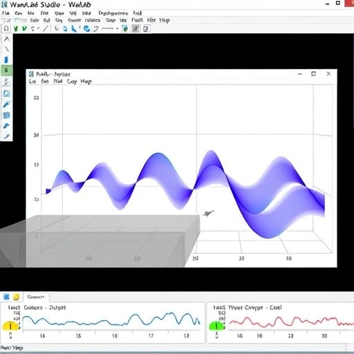
Researchers have unveiled a lightweight, open-source software tool designed to make two-dimensional wave-propagation experiments accessible to students, educators, and researchers who need reproducible scientific workflows without the steep learning curve of full-scale electromagnetic solvers. The tool, called WaveLab Studio, is described in a paper published in the journal SoftwareX, and it arrives at a time when demand for intuitive simulation environments is growing across wireless communication, radar modeling, geophysics, electromagnetic compatibility, and engineering education.

Developed by Kristina Yurlova, Marek Ružička, and Juraj Gazda, WaveLab Studio occupies a deliberately modest but strategically important niche in the simulation software ecosystem. The team is careful to position the tool below production-grade electromagnetic solvers in terms of physical fidelity. Established frameworks such as Meep, gprMax, and openEMS provide high-fidelity finite-difference time-domain modeling of electromagnetic phenomena, while general numerical and scientific machine-learning platforms like FEniCS, DeepXDE, and NVIDIA’s Modulus/PhysicsNeMo support broader partial differential equation and physics-informed neural network workflows. What these systems do not offer, the authors argue, is a compact, low-friction environment in which a user can sketch a heterogeneous scene, inspect it visually, execute it from the command line or a cloud capsule, and receive a standardized package of plots, arrays, and metrics without stitching together several separate scripts.

The technical core of WaveLab Studio is a Python research-software package with three coordinated components: a graphical user interface, a command-line solver, and a set of visualization utilities. The desktop scene builder is implemented with Tkinter, allowing users to set source coordinates and frequency parameters, define material objects, edit geometry, and preview scenes interactively. The solver component, solver_simple_torch.py, runs headless and is built on NumPy and PyTorch, with Matplotlib handling visualization and PyYAML managing configuration. The entire package is distributed under the MIT License, with the current version numbered v0.1.1 and hosted on GitHub.

At the heart of the workflow is a deliberate architectural decision: the YAML file serves as the serialization contract between every interface. A scene file contains a source block storing coordinates, frequency, and amplitude, along with an objects list where each entry specifies a material label, geometric shape, position, size parameters, and optional rotation. A top-level materials mapping can override default parameters such as wave speed, absorption, and transmission. Because the same YAML file can be opened in the graphical interface, inspected with the scene_cli.py tool, executed with the headless solver, and used in a Code Ocean capsule, the tool guarantees that a scenario designed on a desktop produces identical results when run automatically. This cross-interface consistency is the property the authors identify as the tool’s principal contribution.

The default solver operates on a rectangular two-dimensional domain, discretized into a grid whose resolution the user controls through command-line arguments. For each grid point, the algorithm samples the line segment connecting the source to that point and blends material parameters along the segment using soft object-membership masks. The ray-marched field component accumulates a phase term proportional to frequency divided by local wave speed and an exponential attenuation term governed by local absorption, multiplied by a transmission factor. The model then applies a geometric occlusion and shadow map for barrier-like objects, adds a local edge-wave term around obstacle boundaries, and performs an FFT-based smoothing step. An internal quality parameter controls ray sampling density, shadow sampling, smoothing, and edge-effect strength, giving users a continuous dial between speed and visual refinement.

One of the more technically honest aspects of the paper is its treatment of the reference and error metrics. The reference field displayed in figures is not an external physical ground truth but rather the highest-quality internal field produced by the pipeline at its maximum quality setting. The approximated field is computed by the same deterministic pipeline at a lower quality factor, derived from the requested epoch count. The error map, mean absolute error, and maximum absolute error reported by the software are therefore internal consistency measures that indicate how the workflow behaves under different scenes and settings. The authors explicitly state that these metrics are not validation errors against Maxwell-equation solutions, measured data, or independent finite-difference or finite-element solvers. Material names such as concrete, water, and plastic are user-facing labels mapped to scalar parameters and display overlays, and they should be interpreted as graphical and algorithmic scene effects rather than calibrated constitutive electromagnetic constants.

This framing shapes the validity domain of the tool. The solver is a scalar visual propagation model intended for two-dimensional demonstrations. It does not model vector electromagnetic polarization, impedance-matched interface conditions, full material constitutive laws, or perfectly matched absorbing boundaries. The authors argue that this limitation is precisely what makes the software valuable: by keeping the physical model simple, the entire workflow remains fast, transparent, and reproducible, running each illustrative scenario in under three seconds on a CPU-only setup.

To demonstrate the workflow, the repository ships with four YAML scenarios. The first is a free-space baseline with no objects, completing in 2.49 seconds. The second introduces a single concrete obstacle to illustrate shadowing and error-map generation, taking 2.64 seconds. The third presents a heterogeneous multi-material scene with four objects, exercising multi-object interaction in 2.74 seconds, and the fourth compares water and plastic materials to show material-dependent field changes in 2.59 seconds. Each scenario follows the same execution chain: parse the YAML file, build the grid and object masks, run the scalar solver, write a result directory, export field plots, save arrays, and store metrics. Every output set contains the internal reference field, the approximated field, and an absolute error map in a repeated layout, which the authors note is useful for checking whether source position, object geometry, and material labels were preserved across the YAML, command-line, and export stages.

Beyond the default solver, WaveLab Studio includes a preparatory pathway toward physics-informed neural networks. The current release provides the shared scene representation, field-export mechanism, and backend separation needed to prepare neural PDE experiments, but the authors are explicit that they do not claim a validated neural solver. In a future release, the default approximation stage could be replaced by a neural approximation trained with residual, boundary-condition, initial-condition, and data terms, following the general physics-informed neural network framework introduced by Raissi and colleagues in 2019. The present contribution is therefore described as a PINN-ready workflow interface rather than a demonstrated PINN benchmark, a distinction that reflects a growing trend in the literature on physics-informed learning for electromagnetic materials, discontinuous media, and transient two-dimensional fields.

The educational impact of the tool may prove to be its most immediate application. Students can experiment with source position, frequency, material labels, and object geometry without writing a complete simulation program, while the YAML representation exposes the same scene in machine-readable form, helping learners connect visual modeling with reproducible scientific computing practices. In research and thesis-supervision settings, the software supports rapid scenario generation and result packaging: a saved experiment can contain the input scene, numerical outputs, plots, animations, and metrics needed to discuss a simulation result. The authors suggest the tool is well suited to preparing demonstration cases, testing plotting and data-processing scripts, and organizing small scene collections before moving to validated solvers such as Meep, openEMS, or gprMax.

The software is distributed as a Python repository including the GUI entry point, command-line scene tools, example YAML scenes, documentation, smoke tests, and a reproducible Code Ocean capsule that executes the headless path, since the Tkinter interface requires a display server. The code is tested on Linux and Windows-compatible Python environments, and the developers provide support through a contact email listed in the repository documentation.

Looking forward, the team outlines an ambitious development roadmap: benchmark validation against analytical and established solver references, a documented and tested PINN/Modulus backend, improved package modularity, public API documentation, and extension to three-dimensional scene construction with volumetric visualization. For now, WaveLab Studio stands as a demonstration that reproducibility in scientific computing does not always require heavyweight infrastructure. By unifying graphical design, transparent configuration, headless execution, and packaged outputs under a single scene contract, the tool lowers the barrier to entry for wave-propagation experimentation while leaving a clean migration path toward the high-fidelity and machine-learning-based methods that production research ultimately demands. In a field where the gap between classroom demonstrations and research-grade simulation has often been wide, a deliberately simple tool with a rigorous workflow discipline may prove to be exactly the bridge that students and early-stage researchers need.