New Digital Map Divides Earth’s Land Into 20 Subbiomes for Climate Tracking

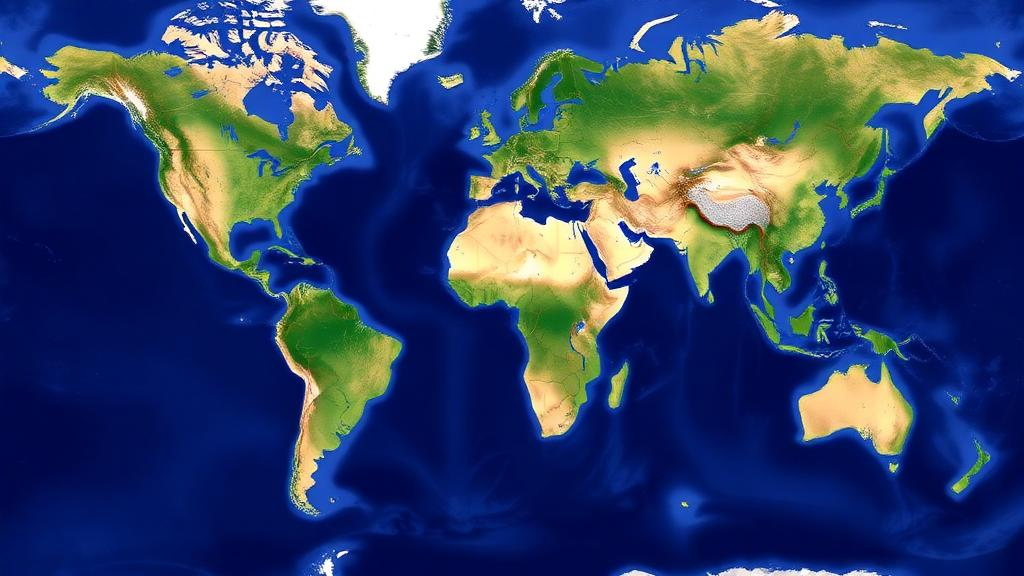
For the first time, scientists have assembled a complete digital vector map that divides every square kilometer of Earth’s land surface into a single, hierarchical system of biotic units. The map, published in the journal Vegetation Classification and Survey, organizes the terrestrial world into four domains, seven ecozones, nine biomes and twenty subbiomes, and it is being released as an open geographic dataset that any researcher can download and analyze. Its creators hope it will become a standard reference for studying global biodiversity patterns and for monitoring how climate change reshapes the living surface of the planet.

The new map is the cartographic companion to a classification scheme presented a year earlier by the same research team, led by vegetation scientist Javier Loidi and colleagues. In that earlier work, the team proposed a comprehensive typology of biomes in the broad sense, meaning large units of ecosystems defined by the interplay of climate and vegetation rather than by political borders or single taxonomic groups. The classification was designed to explain and understand the general patterns of biodiversity across the entire terrestrial area of the planet, including regions such as Antarctica’s ice-free margins and high mountain belts that many global vegetation maps simply leave blank. The new publication turns that conceptual framework into a set of GIS vector layers that can be queried, measured and overlaid with other geospatial data.

Technically, the map consists of polygons drawn manually in the open-source QGIS software environment, a labor-intensive process in which the authors delineated boundaries between biotic units based on climatic and vegetational criteria. The layers are distributed in a zip archive containing four widely used formats: GeoJSON, ESRI shapefile, Keyhole Markup Language (KML) and a QGIS layer settings file. The coordinate reference system is EPSG:4326, also known as WGS 84, the standard latitude-longitude system used by GPS devices and most web mapping platforms, and the character encoding is UTF-8, ensuring that unit names display correctly in any compatible software. This choice of formats and projection means the dataset can be loaded directly into commercial GIS packages, free tools such as QGIS, and even browser-based platforms like Google Earth.

Every polygon in the map carries a rich attribute table, which is what transforms a simple drawing into an analytical instrument. Each feature is tagged with a unique polygon identifier, a code for its subbiome, biome, ecozone and domain, and the human-readable name of each of those units. Critically, the table also stores the area of every polygon in square kilometers, calculated in a World Cylindrical Equal Area projection, designated ESRI:54034. Equal-area projections are essential for this kind of work because they preserve true relative sizes, whereas the more familiar Mercator-style projections distort areas dramatically toward the poles and would make any comparison of unit extents meaningless. Because the hierarchy is embedded in the attributes, a user can dissolve the polygons upward to produce maps at any of the four levels, from the twenty finest subbiomes to the four broadest domains.

The hierarchy itself reflects the dominant climatic forces that shape life on land. At the top sit four domains named for the climatic regimes that govern them. The Cryocratic Domain covers the cold climates, dominated by low temperatures and frozen conditions; the Mesocratic Domain covers temperate climates, including the cool climates of tropical mountains; the Xerocratic Domain covers arid climates where water is the limiting factor; and the Thermocratic Domain covers the warm climates of the tropics. Each domain is subdivided into ecozones, which capture finer seasonal rhythms of moisture and temperature, such as the temperate ombroestival ecozone with its summer rains, the temperate aridiestival ecozone with summer drought, and the hypercontinental steppic ecozone of the continental interiors. Ecozones in turn contain biomes, and biomes contain the twenty subbiomes that represent the finest division in the system.

The numbers reveal some striking truths about how the land is apportioned. The single largest subbiome on Earth is the tropical pluviseasonal forests and woodlands, the great belt of seasonally dry tropical forest and savanna woodland that spans parts of South America, Africa, Asia and Australia. It covers 21,532,324.6 square kilometers, or 16.2 percent of the land surface. It is followed by the lowland boreal Taiga at 16,964,468.7 square kilometers, or 12.7 percent, and by the tropical rain forests at 15,042,477 square kilometers, or 11.3 percent. Together, just three subbiomes account for roughly forty percent of the terrestrial world, a concentration that underscores how strongly climate constrains the distribution of major vegetation types.

Aggregated to the biome level, the tropical pluviseasonal forests and shrublands dominate with 29,576,514.8 square kilometers, or 22.2 percent of the land. The biome of deserts and semi-deserts of arid regions comes second at 26,046,887.6 square kilometers, or 19.6 percent, itself divided into cold, temperate and warm desert subbiomes of similar size, each covering between about 5.5 and 10.4 million square kilometers. The boreal forest biome ranks third at 19,716,082.4 square kilometers, or 14.8 percent. At the highest level, the Thermocratic Domain of warm climates emerges as the largest of the four domains, occupying 33.5 percent of the land surface, ahead of the Mesocratic Domain at 23.7 percent, the Cryocratic Domain at 23.2 percent and the Xerocratic Domain at 19.6 percent.

Some of the rarer units tell their own stories. The conifer coastal forests subbiome, which includes the temperate rainforests of the Pacific coast of North America, covers only 207,387.7 square kilometers, about 0.16 percent of the land, making it among the smallest and most geographically restricted units on the map. The tropical montane cloud lauroid and conifer evergreen forest, found on tropical mountains where orographic clouds bathe the vegetation, spans 2,316,614 square kilometers. Tundras are split into three subbiomes according to latitude and altitude: polar tundra at 7,918,667 square kilometers, tundras of the temperate mountains in the cryoro belt at 2,538,587 square kilometers, and tundras of the tropical mountains at 798,811 square kilometers. This subdivision captures a key ecological insight, that alpine and polar cold climates produce similar vegetation even at vastly different latitudes.

Why does a map like this matter now? The authors point explicitly to climate change monitoring as a primary application. Because the biotic units are defined by climatic conditions, shifts in their boundaries over time can serve as indicators of how warming is redistributing the planet’s life zones. The boreal Taiga and polar tundra, which together with mountain tundras make up the Cryocratic Domain’s 23.2 percent share, are expected to be especially dynamic as temperatures rise, and having a rigorous baseline against which to measure contraction or displacement is a prerequisite for detecting those changes. Conservation planners can also use the map to assess how well protected-area networks represent each subbiome, since rare units such as the conifer coastal forests may deserve proportionally greater attention than their tiny extents currently receive.

The map’s hierarchical design also gives it flexibility that single-level classifications lack. A scientist modeling species distributions might work at the subbiome level to capture fine climatic distinctions, while a global carbon accounting study might aggregate to domains to keep the analysis tractable. Because the dataset is released in open formats with full attribute documentation, it invites reuse in biodiversity assessments, biogeographic research, paleoecological reconstructions and education. By providing a consistent, complete and freely available partition of the terrestrial world, the authors have given the international community a common geographic language for describing ecosystems, one that will only grow more valuable as the climate continues to move the boundaries it draws.

Subject of Research: A global hierarchical vector map of terrestrial biotic units for biodiversity and climate monitoring

Article Title: A vector map of the world’s terrestrial biotic units: subbiomes, biomes, ecozones and domains

Article References: Loidi, J., Navarro-Sánchez, G., & Vynokurov, D. (2023). A vector map of the world’s terrestrial biotic units: subbiomes, biomes, ecozones and domains. Vegetation Classification and Survey, 4, 59-61. https://doi.org/10.3897/vcs.99167

Image Credits: AI Generated

DOI: 10.3897/VCS.99167

Keywords: biomes, subbiomes, ecozones, biotic units, vegetation classification, GIS vector map, climate change monitoring, biodiversity, taiga, tropical forests, tundra, global ecology